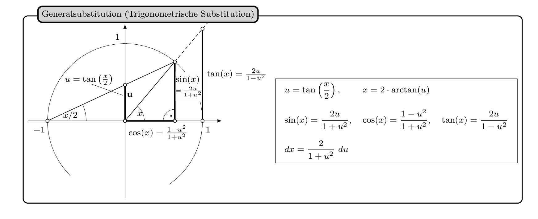
Folgender Plot zeigt eine Übersicht der sogen. Generalsubstitution, zum Lösen von Integralen des Typs ∫f(sin(x), cos(x), tan(x))dx
Die Winkelbezeichnungen habe ich dabei, um rasch ein TikZ-Bild zu erstellen, nach Augenmaß gesetzt.
Wer es professionell machen möchte, kann hier schauen:
Wie setze ich am besten die Winkelbeschriftung bei selbstgezeichneten Winkeln?
(Klicke auf das Bild)
\documentclass[margin=5mm]{standalone}
%\documentclass[a5paper, landscape]{scrartcl}
\usepackage[ngerman]{babel}
\usepackage{tikz}
\usetikzlibrary{calc, backgrounds}
\usepackage{amsmath, amssymb}
% \pagecolor{olive!50!yellow!50!white}
%===========
\begin{document}
%===========
\def\scala{2.5}
\tikzstyle{background rectangle}=
[thick,draw=black, fill=white, rounded corners]
\begin{tikzpicture}[show background rectangle, >=latex, font=\footnotesize, scale=\scala]
%Koordinaten
\coordinate (O) at (0,0);
\coordinate (L) at ($({cos(50)},{0})$);
\coordinate (P) at ($({cos(50)},{sin(50)})$);
\coordinate (Q) at (-1,0);
\coordinate (U) at ($({0},{tan(50/2)})$);
\coordinate (U1) at (-0.5,0.5);
\coordinate (U2) at ($({0},{tan(50/2)/2})$);
\coordinate (T) at ($({1},{tan(50)})$);
\coordinate (F) at (1,0);
%Einheitskreisbogen
\draw[very thin] ([shift=(-55:1)]O) arc (-55:225:1); %Bogen mit Zentrum (0,0)
%Strecken
%Koordinatensystem:
\draw[thin, ->] (-1.25,0) — (1.25,0) node[]{$$};
\draw[thin, ->] (0,-1.0) — (0,1.25) node[]{$$};
\draw[] (1,2pt/\scala) — (1,-2pt/\scala) node[right=5pt, below]{$1$};
\draw[] (-1,2pt/\scala) — (-1,-2pt/\scala) node[left=7.5pt, below]{$-1$};
\draw[] (2pt/\scala,1) — (-2pt/\scala,1) node[left=5pt, above]{$1$};
%Radius
\draw[] (O) — (P) node[midway, below, sloped]{$$};
%Hilfslinie
\draw[] (Q) — (P) node[]{$$};
%tan x/2
\draw[very thick] (O) — (U) node[midway, right, yshift=7.5pt, xshift=-2.5pt]{$\mathbf{u}$};
\draw[very thin, shorten >=2.0pt, shorten <=4.5pt] (U1)–([yshift=2.5pt]U2) node[above=-6pt, pos=0, xshift=2.5pt]{$u = \tan\left(\frac{x}{2}\right)$};
%cos
\draw[very thick] (O) — (L) node[midway, below, xshift=7.5pt]{$\cos(x)=\frac{1-u^2}{1+u^2}$};
%sin
\draw[very thick] (P) — (L) node[fill=white!99!black, align=left, midway, right=-3pt, yshift=4.5pt]{$\sin(x)$ \\ \tiny$=\!\frac{2u}{1+u^2}$};
\draw[very thick] (P) — (L);
%tan:
\draw[very thick] (T) — (F) node[midway, right]{$\tan(x) = \frac{2u}{1-u^2}$};
\draw[densely dashed,shorten >= -10pt] (P) — (T) node[]{$$};
%Winkel
\draw[very thin] ([shift=(0:0.25)]O) arc (0:50:0.25) node[left=-2pt, below=2pt]{$x$};
\draw[very thin] ([shift=(0:0.5)]Q) arc (0:25:0.5) node[xshift=-0.4cm, yshift=-0.35cm]{$x/2$};
%Hilfswinkel
%\draw[very thin] ([shift=(205:0.4)]P) arc (205:230:0.4) node[xshift=0.15cm, yshift=0.4cm]{$\varrho$};
%\draw[<->, very thin] ([shift=(50:0.25)]O) arc (50:180:0.25) node[xshift=0.0cm, yshift=0.5cm]{$\chi$};
\draw[very thin] ([shift=(90:0.15)]L) arc (90:180:0.15) node[xshift=0.25cm, yshift=0.15cm]{\Large$\cdot$};
%Punkte
\draw[] plot[mark=*, mark size=1.5pt/\scala, mark options={fill=white}] coordinates{(O)} node[left=5pt, below]{$$};
\draw[] plot[mark=*, mark size=1.5pt/\scala, mark options={fill=white}] coordinates{(L)} node[left]{$$};
\draw[] plot[mark=*, mark size=1.5pt/\scala, mark options={fill=white}] coordinates{(P)} node[above]{$$};
\draw[] plot[mark=*, mark size=1.5pt/\scala, mark options={fill=white}] coordinates{(Q)} node[above=5pt, left]{$$};
\draw[] plot[mark=*, mark size=1.5pt/\scala, mark options={fill=white}] coordinates{(U)} node[below=5pt, right]{$$};
\draw[] plot[mark=*, mark size=1.5pt/\scala, mark options={fill=white}] coordinates{(T)} node[below=5pt, right]{$$};
\draw[] plot[mark=*, mark size=1.5pt/\scala, mark options={fill=white}] coordinates{(F)} node[below=5pt, right]{$$};
%Infobox
\node[draw] at (3.5,0) {$%
\begin{array}{lll}
u = \tan\left(\dfrac{x}{2}\right), & x = 2 \cdot \arctan(u) & \\ \\
\sin(x) = \dfrac{2u}{1+u^2},
& \cos(x) = \dfrac{1-u^2}{1+u^2},
& \tan(x) = \dfrac{2u}{1-u^2} \\ \\
dx = \dfrac{2}{1+u^2} ~ du
\end{array}
$};
%Überschrift
\node [xshift=2ex,yshift=-0.5ex,overlay,very thick, draw=black, fill=lightgray!80,rounded corners,above right] at (current bounding box.north west){ Generalsubstitution (Trigonometrische Substitution) };
\end{tikzpicture}
%===========
\end{document}
%===========
Comments
4 responses to “Trigonometrische Substitution”
Irgendwas ist beim Code schiefgegangen – es hat viele Leerzeilen gesetzt 🙁
Du kannst LaTeX-Code einfach zwischen
[cce lang="latex"]...[/cce]posten. Dann sieht alles normal aus. Dazu solltest Du den Editor aber wahrscheinlich von HTML auf Text umstellen.Ach Mann, ja diese HTML-Ansicht hat mir die ganzen Leerzeilen reingemacht. Diese Autoformate sind nicht im Sinne des TeX-Nutzers :()
Ja, WordPress ist da leider eigenmächtig. Und es frisst führende Leerzeichen, es sei denn, es ist
-formatierter Code. Ich habe extra das Codecolorer-Plugin modifiziert, dass es enthaltene pre-Tags nicht mit ausgibt. Es funktioniert also ohne Probleme:
Das “überlebt” auch den visuellen Editor. So ist es auch in Deinem ersten Beitrag. Danke für die schönen Beispiele!